Introduction
Child Neglect as a Public Health Issue
Lots of stuff here about neglected children…
The objective of this tutorial: 1. Code, data for paper in progress 2. Use supervised machine learning to predict new cases of child neglect
Data Source
Methodology
# Base URL path
library(RSocrata)
library(tidyverse)
## ── Attaching packages ───────────────────────────────────────────────────────────────────────────────────────────────────────── tidyverse 1.2.1 ──## ✔ ggplot2 3.2.0 ✔ purrr 0.3.2
## ✔ tibble 2.1.3 ✔ dplyr 0.8.3
## ✔ tidyr 0.8.3 ✔ stringr 1.4.0
## ✔ readr 1.3.1 ✔ forcats 0.4.0## ── Conflicts ──────────────────────────────────────────────────────────────────────────────────────────────────────────── tidyverse_conflicts() ──
## ✖ dplyr::filter() masks stats::filter()
## ✖ dplyr::lag() masks stats::lag()library(dplyr)base_url = "https://data.lacity.org/resource/63jg-8b9z.json?"
#7749esl6s83yobtq1033yn1gq -- ID
#3bpoe7q2jkpodx0025841q59ct6asvpwgyzlpwuijqxlec95fb -- secret
my_token <- "w0BkWUPZYzjQRwNEVX8KEijw4"
fdf <- read.socrata(base_url, my_token)
#secret token 6epp7RDgzqjARarbW5EpUEJm-ZPFe1-EROQK
glimpse(fdf)## Observations: 2,002,224
## Variables: 28
## $ dr_no <chr> "001307355", "011401303", "070309629", "090631215…
## $ date_rptd <dttm> 2010-02-20, 2010-09-13, 2010-08-09, 2010-01-05, …
## $ date_occ <dttm> 2010-02-20, 2010-09-12, 2010-08-09, 2010-01-05, …
## $ time_occ <chr> "1350", "0045", "1515", "0150", "2100", "1650", "…
## $ area <chr> "13", "14", "13", "06", "01", "01", "01", "01", "…
## $ area_name <chr> "Newton", "Pacific", "Newton", "Hollywood", "Cent…
## $ rpt_dist_no <chr> "1385", "1485", "1324", "0646", "0176", "0162", "…
## $ part_1_2 <chr> "2", "2", "2", "2", "1", "1", "1", "1", "1", "1",…
## $ crm_cd <chr> "900", "740", "946", "900", "122", "442", "330", …
## $ crm_cd_desc <chr> "VIOLATION OF COURT ORDER", "VANDALISM - FELONY (…
## $ mocodes <chr> "0913 1814 2000", "0329", "0344", "1100 0400 1402…
## $ vict_age <chr> "48", "0", "0", "47", "47", "23", "46", "51", "30…
## $ vict_sex <chr> "M", "M", "M", "F", "F", "M", "M", "M", "M", "M",…
## $ vict_descent <chr> "H", "W", "H", "W", "H", "B", "H", "B", "H", "W",…
## $ premis_cd <chr> "501", "101", "103", "101", "103", "404", "101", …
## $ premis_desc <chr> "SINGLE FAMILY DWELLING", "STREET", "ALLEY", "STR…
## $ status <chr> "AA", "IC", "IC", "IC", "IC", "AA", "IC", "AA", "…
## $ status_desc <chr> "Adult Arrest", "Invest Cont", "Invest Cont", "In…
## $ crm_cd_1 <chr> "900", "740", "946", "900", "122", "442", "330", …
## $ location <chr> "300 E GAGE AV", "SEPULV…
## $ lat <chr> "33.9825", "33.9599", "34.0224", "34.1016", "34.0…
## $ lon <chr> "-118.2695", "-118.3962", "-118.2524", "-118.3295…
## $ cross_street <chr> NA, "MANCHESTER AV", NA, "HOLLY…
## $ weapon_used_cd <chr> NA, NA, NA, "102", "400", NA, NA, "500", "400", N…
## $ weapon_desc <chr> NA, NA, NA, "HAND GUN", "STRONG-ARM (HANDS, FIST,…
## $ crm_cd_2 <chr> NA, NA, NA, "998", NA, NA, NA, NA, NA, "998", NA,…
## $ crm_cd_3 <chr> NA, NA, NA, NA, NA, NA, NA, NA, NA, NA, NA, NA, N…
## $ crm_cd_4 <chr> NA, NA, NA, NA, NA, NA, NA, NA, NA, NA, NA, NA, N…## [1] "list"The following code transforms the age variable from character to numeric and filters the victim’s age to be between 6 and 12. Then, it searches the crime descriptions for the word “child.” Finally, we plot a histogram of victim’s age.
childcrimes <- fdf %>%
  mutate(vict_age = as.numeric(vict_age)) %>%
  filter(vict_age >=6 & vict_age < 13) %>%
  filter(str_detect(crm_cd_desc, 'Child|CHILD|child'))

ggplot(childcrimes, mapping = aes(vict_age)) + geom_bar()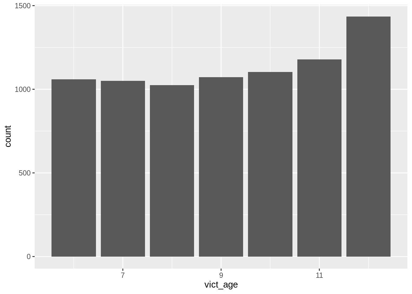
What Neighborhoods Have the Most Child Crimes?
First, we count the number of total crimes
## # A tibble: 8 x 2
##   crm_cd_desc                                     n
##   <chr>                                       <int>
## 1 CHILD ABANDONMENT                              26
## 2 CHILD ABUSE (PHYSICAL) - AGGRAVATED ASSAULT   518
## 3 CHILD ABUSE (PHYSICAL) - SIMPLE ASSAULT      3814
## 4 CHILD ANNOYING (17YRS & UNDER)               1740
## 5 CHILD NEGLECT (SEE 300 W.I.C.)               1674
## 6 CHILD PORNOGRAPHY                              14
## 7 CHILD STEALING                                 32
## 8 LEWD/LASCIVIOUS ACTS WITH CHILD               108
Then, we group the crimes by neighborhood and count the number of crimes by neighborhood.
crimebyarea <-  childcrimes  %>%
  dplyr::group_by(crm_cd_desc, area_name) %>%
  dplyr::summarise(count= n())

crimebyarea <- na.omit(crimebyarea)

wide_crimebyarea <- crimebyarea %>% spread(key = area_name, value = count)
wide_crimebyarea[is.na(wide_crimebyarea)] <- 0
wide_crimebyarea$total_col = apply(wide_crimebyarea[,-1], 1, sum)
wide_crimebyarea$percent_Mission <- wide_crimebyarea$Mission / wide_crimebyarea$total_col
Now we can plot the neighborhood with the most crimes by type of crime.
ggplot(wide_crimebyarea, aes(x= reorder(crm_cd_desc, percent_Mission),
  y = percent_Mission, fill = percent_Mission, group = 1)) +
  geom_bar(stat = "identity") +
  ylab("Percentage of All Crimes") +
  xlab("Crime Subtypes") + scale_x_discrete(labels = c("CHILD ABANDONMENT" = "CA",
                                        "CHILD ABUSE (PHYSICAL) - AGGRAVATED ASSAULT" = "PAAGG",
                                        "CHILD ABUSE (PHYSICAL) - SIMPLE ASSAULT" = "PASA",
                                        "CHILD ANNOYING (17YRS & UNDER)" = "ANNOY",
                                        "CHILD NEGLECT (SEE 300 W.I.C.)" = "NEG",
                                        "CHILD PORNOGRAPHY" = "PORN",
                                        "CHILD STEALING" = "STEAL",
                                        "LEWD/LASCIVIOUS ACTS WITH CHILD" = "CSA")) +
  labs(title = "Crimes Against Children Aged 6-12 in Mission Hills",
       subtitle = "2010 - 2018, City of Los Angeles")+
  theme(axis.text.x = element_text(size=12))+
  theme(axis.text.y = element_text(size = 12))+
  theme(axis.title.x = element_text(size=12,color = "#424242"))+
  theme(axis.title.y = element_text(size = 12,color = "#424242"))+
  theme(plot.title = element_text(lineheight=3, color="black", face = "bold", size=16, hjust =0.5),
        plot.subtitle=element_text(size=14, hjust = 0.5))
The abbreviations for these crimes are as follows…. We see that about 12% of children who were abandoned were in the neighborhood of Mission Hills.
Note that the
The abbreviations for these crimes are as follows…. We see that about 12% of children who were abandoned were in the neighborhood of Mission Hills.
Note that the echo = FALSE parameter was added to the code chunk to prevent printing of the R code that generated the plot.